This guide will demonstrate how you can use gadgetr to set up and run a simple short-cut (no assessment) management strategy evaluation (MSE) using a gadget model as an Operating Model (OM).

Installing the package

As for now, the package is yet to find its way into CRAN. However, you can use our alternative repo that enables you to use R’s install.packages():

install.packages("gadgetr", repos = "https://redus-imr.github.io/gadget")

Or, you can download and install from the pre-compiled binaries here:

https://github.com/REDUS-IMR/gadget/releases/latest

Or, you might want to compile it from the source available in Github:

devtools::install_github("REDUS-IMR/gadget", ref="gadgetr")

The main code

To facilitate parallel runs, the whole MSE codes are encapsulated in a function called runPMSE():

runPMSE <- function(seed = 1234) {

Loading the package

Load the package as usual using the command below.

library(gadgetr)

Loading the example model

We will use the example haddock model. For this purpose, we use the model fitted to the historical period (1978–1999) and project 21-year forecasts (2000–2020) by extending the simulation years in the gadget model.This means that the model end time parameter (lastyear) is set to 2020.

# Get the path of the example haddock model
exPath <- gadgetr::loadExample()
print(exPath)

# Initiate the haddock model
gadgetr::initGadget(exPath, "refinputfile")

# Print the basic model information
gadgetr::getEcosystemInfo()

# Init seed
set.seed(seed)

Defining helper functions

For this simple demonstration, we create four helper functions for MSE simulations; 1) a function to calculate SSB, 2) a function to extract recruit numbers, 3) a function to forecast recruitment, and 4) a function to calculate TAC.

1) Calculating SSB

This function calculates the spawning stock biomass (SSB) for a given stock. Here we assume that individuals of 3-year-olds and older are mature and only stock information in step 4 will be taken into the calculation.

# Calculate SSB
calcSSB <- function(stk) {
    # Get SSB
    subs <- stk[stk[, "age"] >= 3 & stk[, "step"] == 4, ]
    ssb <- sum(subs[, "number"] * subs[, "meanWeights"])
    return(ssb)
}

2) Calculating recruitment

A simple function for calculating the “real” recruitment values (no observation error) for a given stock in a year. Only 1-year-olds are used in the calculation. Because stock information (numbers and weights) is collected after each quarter (step) in simulations, we use the recruitment values from quarter 2.

# Calculate Recruitment
calcRecruitment <- function(stk) {
    # Get Recruitment (based on fbar and only from the last step)
    subs <- stk[stk[, "age"] == 1 & stk[, "step"] == 2, ]
    return(sum(subs[, "number"]))
}

3) Forecasting a recruitment

This function uses the constant recruitment model fit to forecast recruitment.

# In this example, we assume that the haddock recruitment for a given year is
# equal to the historical geometric mean recruitment
fcRecruitment <- function(rec) {
    rec <- unlist(rec)
    return(exp(mean(log(rec))))
}

4) Calculating TAC

We use a simple function to project the next year’s total allowable catch (TAC), assuming that target exploitation rate is 40% of stock biomass in a given year.

# and calculating TAC is a matter of taking 40% of the stock's last year
# stock biomass value with added noise
calcTAC <- function(stk) {
    # Get TSB
    subs <- stk[stk[, "step"] == 4, ]
    tsb <- sum(subs[, "number"] * subs[, "meanWeights"])
    # Calculate error
    err <- rnorm(1, 0, tsb * .25)
    # Calculate TAC
    tac <- .4 * (tsb + err)
    return(tac)
}

Running the hindcast simulation

The haddock model’s hindcast period spans from 1978 to 1999. As the first step, we run gadget until 1999.

# Placeholders for values
stats <- list()
ssb <- list()
rec <- list()

# Loop for the hindcast period
forecastYear <- 2000
status <- gadgetr::getEcosystemInfo()
while ( status[["time"]]["currentYear"] < forecastYear ) {
  # Append stats
  curYr <- as.character(status[["time"]]["currentYear"])
  stats[[curYr]] <- gadgetr::runYear()
  ssb[[curYr]] <- calcSSB(stats[[curYr]]$stock$had$stk)
  rec[[curYr]] <- calcRecruitment(stats[[curYr]]$stock$had$stk)
  # Get the latest runtime information
  status <- gadgetr::getEcosystemInfo()
}

Running the forecast simulation

Now, we run the simulation from year 2000 to 2020. In looping through the years, we also perform the following steps at the beginning of the year (i.e., before quarter (step) 1):

Project recruitment by calling fcRecruitment().
Apply the projected recruitment to the simulation using gadgetr::updateRenewal() on the had stock.
Calculate the last year’s SSB at the beginning of the year using calcSSB().
Calculate TAC for the year using calcTAC().
Apply the calculated TAC to the future total fleet in the gadget simulation using gadgetr::updateAmount().

# MSE loop
while ( status[["time"]]["finished"] != 1 ) {
  # Time calculation
  curYr <- status[["time"]]["currentYear"]
  lastYr <- curYr - 1
  
  # Calculate Recruitment for this year
  recNumber <- fcRecruitment(rec)
  rec[[as.character(curYr)]] <- recNumber
  print(paste("Recruitment in", curYr, "is", recNumber))

  # Apply recruitment number for this year haddock stock
  # note that this is similar to the format found in "had.rec" file
  updateRenewal("had", curYr, step = 1, area = 1, age = 1,
      number = (recNumber/10000), mean = 16.41, sdev = 2.25 , alpha = 8.85e-6,
      beta = 3.0257)

  # Calculate last year SSB
  stk0 <- stats[[as.character(lastYr)]]$stock$had$stk
  ssb[[as.character(lastYr)]] <- calcSSB(stk0)

  # Calculate TAC for this year
  tac <- calcTAC(stk0)
  print(paste("TAC in", curYr, "is", tac))

  # Apply TAC to fleet data (spread out over 4 quarter/step in a year)
  # in percentage (i.e., sum(tacPortion) == 1)
  tacPortion <- c(0.232, 0.351, 0.298, 0.119)
  targetFleet <- "future"
  updateAmount(targetFleet, curYr, 1, 1, tacPortion[[1]] * tac)
  updateAmount(targetFleet, curYr, 2, 1, tacPortion[[2]] * tac)
  updateAmount(targetFleet, curYr, 3, 1, tacPortion[[3]] * tac)
  updateAmount(targetFleet, curYr, 4, 1, tacPortion[[4]] * tac)

  # Forward the time
  stats[[as.character(curYr)]] <- gadgetr::runYear()

  # Get the latest runtime information
  status <- gadgetr::getEcosystemInfo()
}

Summarizing stock status and catch

After the loop finishes, we summarize the main performance metrics.

print(rec)
# Calculate real catch (all fleets)
catch <- lapply(stats, function(x) {
    sum(x$fleet$future$catch$had[, "biomassConsumed"], na.rm = TRUE) +
    sum(x$fleet$comm$catch$had[, "biomassConsumed"], na.rm = TRUE) +
    sum(x$fleet$survey$catch$had[, "biomassConsumed"], na.rm = TRUE)
  })

Ending gadget

After each simulation, it is necessary to properly terminate an active gadget simulation run.

endGadget()

Ending runPMSE

    return(list(ssb, rec, catch))
}

This is the end of the runPMSE() and we return the recruitment, SSB and catch metrics.

Do a single run

Now let’s try to do a single run and plot the output. But first let’s make a plot generator function.

plotIt <- function(x) {
    singlePlot <- function(cat, name, title) {
        # Collect metrics
        z <- do.call(cbind, lapply(x, function(y) unlist(y[[cat]])))
        tab <- as.data.frame(z)
        tab$year <- as.numeric(rownames(tab))
        tab <- reshape(tab, varying=list(1:(ncol(tab)-1)), direction="long", v.names = name)
        fig <- ggplot(tab, aes_string("year", name)) +
                    stat_summary(geom = "line", fun = mean) +
                    stat_summary(geom = "ribbon", fun.data = mean_sdl, fun.args = list(mult = 1), fill = "red", alpha = 0.2) +
                    stat_summary(geom = "ribbon", fun.data = mean_cl_normal, fill = "red", alpha = 0.3) + 
                    labs(title=paste("Haddock", title), y="")
        return(fig)
    }

  ssbplot <- singlePlot(1, "ssb", "SSB")
  recplot <- singlePlot(2, "rec", "Recruitment")
  catchplot <- singlePlot(3, "catch", "Catch")

  return(list(ssbplot, recplot, catchplot))
}

library(ggplot2)
result <- runPMSE()
#> [1] "/home/runner/work/_temp/Library/gadgetr/extdata/haddock"
#> Gadget version 2.2.00-BETA running on fv-az82 Tue Sep 15 12:17:36 2020
#> Starting Gadget from directory: /home/runner/work/_temp/Library/gadgetr/extdata/haddock
#> using data from directory: /home/runner/work/_temp/Library/gadgetr/extdata/haddock
#> 
#> Finished reading model data files, starting to run simulation
#> [1] "Gadget is started with the given model in /home/runner/work/_temp/Library/gadgetr/extdata/haddock."
#> [1] "Recruitment in 2000 is 86952975.652955"
#> [1] "TAC in 2000 is 44257236.5811536"
#> Step is 89
#> Change fleet "future" - Step: 89 - Area: 1 with 1.02677e+07
#> Value before 0
#> Value after 1.02677e+07
#> Step is 90
#> Change fleet "future" - Step: 90 - Area: 1 with 1.55343e+07
#> Value before 0
#> Value after 1.55343e+07
#> Step is 91
#> Change fleet "future" - Step: 91 - Area: 1 with 1.31887e+07
#> Value before 0
#> Value after 1.31887e+07
#> Step is 92
#> Change fleet "future" - Step: 92 - Area: 1 with 5.26661e+06
#> Value before 0
#> Value after 5.26661e+06
...

Plotting the result

Generate the performance metric plots.

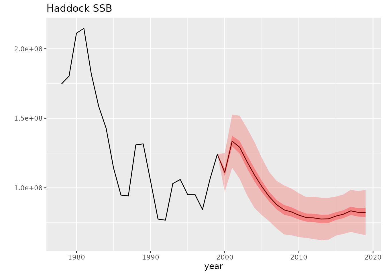
plots <- plotIt(list(result))
print(plots[[1]])
#> Warning in max(ids, na.rm = TRUE): no non-missing arguments to max; returning -
#> Inf

#> Warning in max(ids, na.rm = TRUE): no non-missing arguments to max; returning -
#> Inf

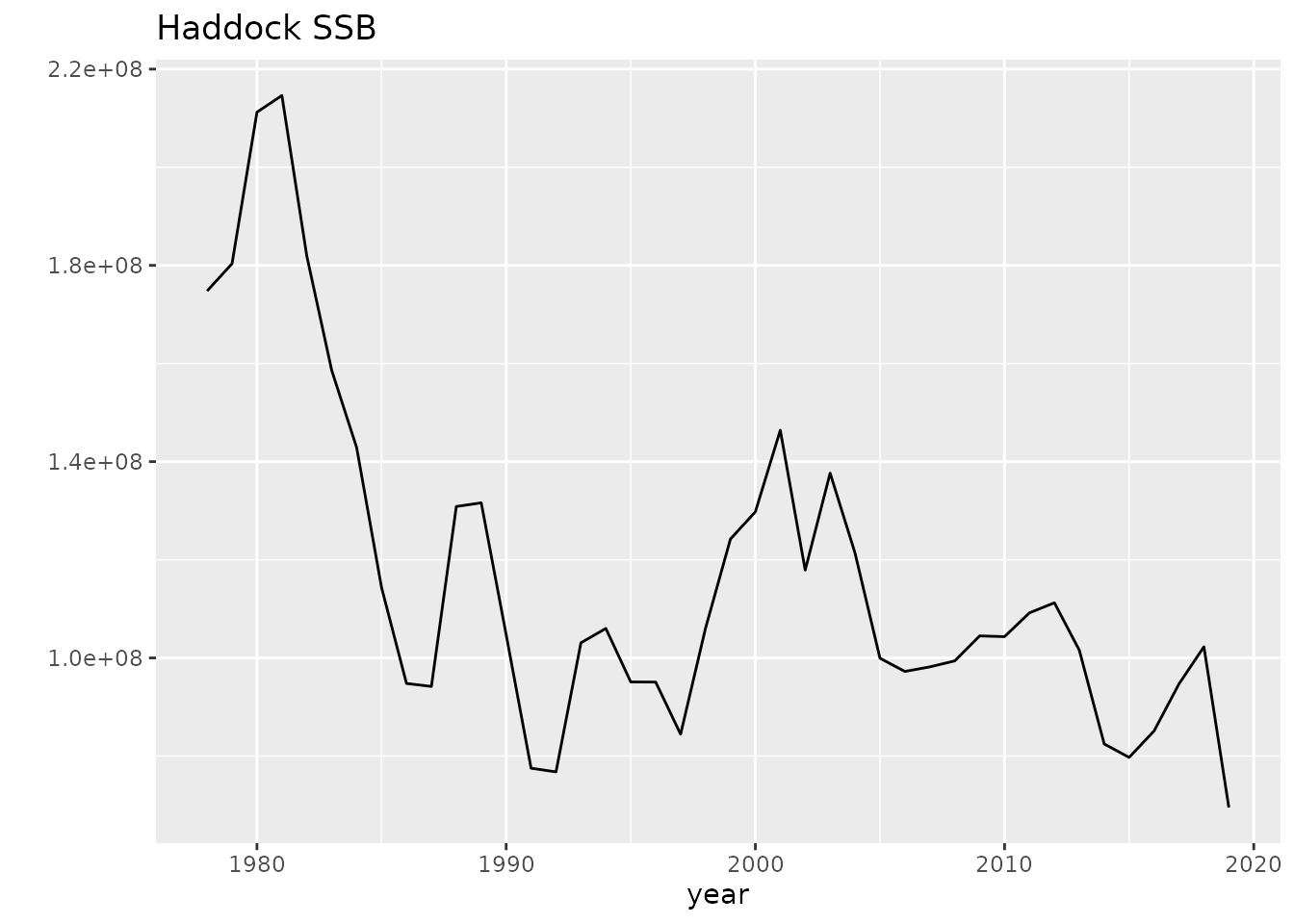
Haddock model (single-run) performance metrics

print(plots[[2]])
#> Warning in max(ids, na.rm = TRUE): no non-missing arguments to max; returning -
#> Inf

#> Warning in max(ids, na.rm = TRUE): no non-missing arguments to max; returning -
#> Inf

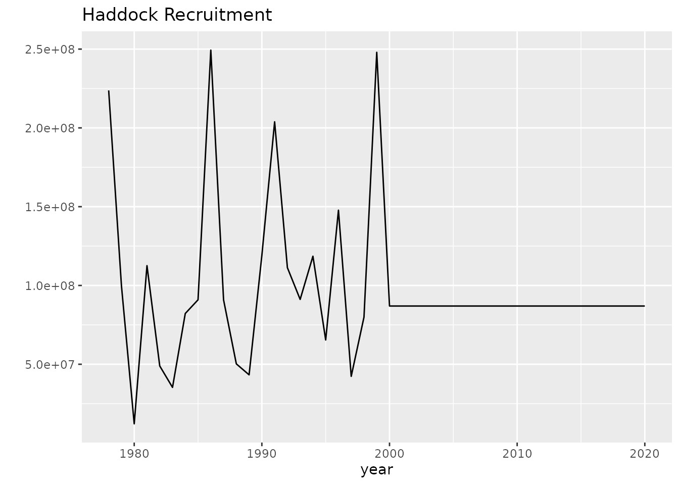
Haddock model (single-run) performance metrics

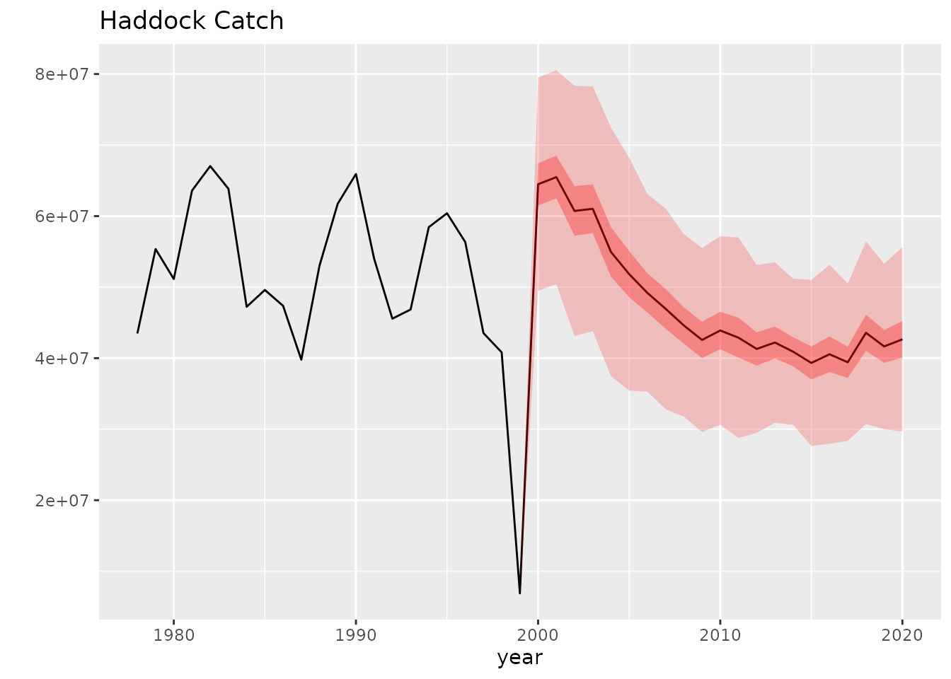
print(plots[[3]])
#> Warning in max(ids, na.rm = TRUE): no non-missing arguments to max; returning -
#> Inf

#> Warning in max(ids, na.rm = TRUE): no non-missing arguments to max; returning -
#> Inf

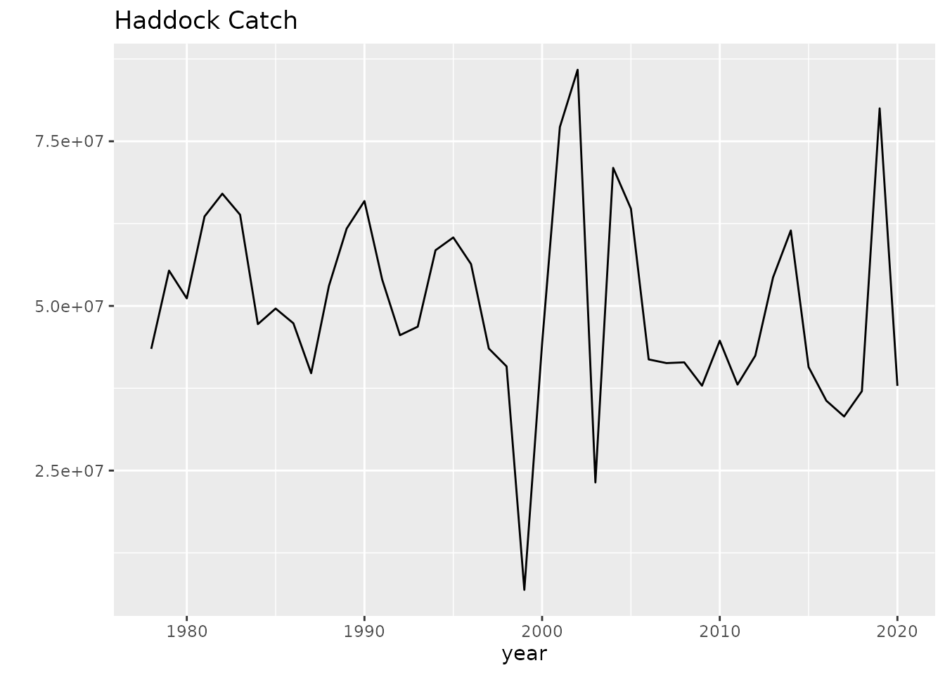
Haddock model (single-run) performance metrics

Do multiple runs in parallel

Here is an example of doing a multiple iteration runs utilizing the R parallel execution capability.

library(parallel)

chk <- Sys.getenv("_R_CHECK_LIMIT_CORES_", "")

if (nzchar(chk) && chk == "TRUE") {
    # use 2 cores in CRAN/actions
    num_workers <- 2L
} else {
    # use all cores in devtools::test()
    num_workers <- detectCores()
}

cl <- makeCluster(num_workers, type = "PSOCK")

# Run
seeds <- round(runif(100, 1, 10000))
result <- parLapply(cl, seeds, runPMSE)

stopCluster(cl)

plots <- plotIt(result)

Plotting the result

Plot the performance metrics from the runs.

print(plots[[1]])

Haddock model (parallel-runs) performance metrics

print(plots[[2]])

Haddock model (parallel-runs) performance metrics

print(plots[[3]])

Haddock model (parallel-runs) performance metrics

GadgetR: (Very) Simple short-cut Management Strategy Evaluation (MSE) using Gadget as the Operating Model (OM)

Ibrahim Umar

2020-09-15

Installing the package

The main code

Loading the package

Loading the example model

Defining helper functions

1) Calculating SSB

2) Calculating recruitment

3) Forecasting a recruitment

4) Calculating TAC

Running the hindcast simulation

Running the forecast simulation

Summarizing stock status and catch

Ending gadget

Ending runPMSE

Do a single run

Plotting the result

Do multiple runs in parallel

Plotting the result