GadgetR: Gadget and FLR Example
Ibrahim Umar
2020-09-15
gadget-flr.RmdAbout FLR capability of GadgetR
The FLR project ([https://flr-project.org]) is a collection of fisheries library in R that provide a set of tools for quantitative fisheries science.
GadgetR has a built-in automatic FLR objects generator feature when running a model simulation. This interoperability enables users to utilize the wealth of useful tools that the FLR suite offers when running a Gadget model simulation.
This guide will demonstrate a simple scenario of how to run a simple short-cut (no assessment) management strategy evaluation (MSE) using a gadget model as an Operating Model (OM). The management loop, especially the recruitment forecast and total allowable catch determination are calculated using several tools that FLR provides (e.g., (FLSR)[https://flr-project.org/doc/Modelling_stock_recruitment_with_FLSR.html] for the modelling of stock-recruitment). This MSE code also utilizes several different stock-recruitment models running in parallel to investigate the possible uncertainty sources during the simulated management process.
Installing the package
As for now, the package is yet to find its way into CRAN. However, you can use our alternative repo that enables you to use R’s install.packages():
install.packages("gadgetr", repos = "https://redus-imr.github.io/gadget")Or, you can download and install from the pre-compiled binaries here:
https://github.com/REDUS-IMR/gadget/releases/latestOr, you might want to compile it from the source available in Github:
devtools::install_github("REDUS-IMR/gadget", ref="gadgetr")
(Very) simple MSE with GadgetR and FLR
Setting up the parameters
First we need to define several parameters that will aid the conversion from gadget output into the FLR objects. This parameters need to be carefully tuned and reflects the actual gagdet model parametes.
# Set simulation time parameters
firstYear <- 1978
projYear <- 2000
finalYear <- 2020

# Set up a stock (or stocks) for Gadget
## List all the unique species
#stockList <- c("had", "cod")
stockList <- c("had")

# HAD
## List all the fleets for all the species
had.fleets <- c("comm", "survey", "future")

## List all the different stock category for had
had.stocks <- c("had")

## List all the mature stock category for had
had.stocks.mature <- c("had")

## List the survey fleets for had
had.surveys <- c("survey")

## List the forecast fleets for had
had.forecasts <- c("future")

## Set stock parameters for the OM
# m2 = NULL means we calculate m2 from gadget result, m2 = 0 means we use only
#      residual mortality (m1)
# StockStep: in which step we should observe the stock number
had.params <- list(stockStep = 2, minage = 1, maxage = 10, minfbar = 2, maxfbar = 8,
                   startf = 0.56, endf = 0.65, areas = c(1), m1 = c(0.2), m2 = NULL)

# COD (if applicable)
#cod.fleets <- c("cod.comm", "cod.survey")
#cod.stocks <- c("cod")
#had.params <- list(stockStep = 2, minage = 1, maxage = 8, minfbar = 4, maxfbar = 8,
#                   startf = 0.56, endf = 0.65, areas = c(1), m1 = c(0.2), m2 = NULL)
#...
After writing the above (exhaustive) parameters, we need a helper function that can convert the parameters into a list object that gagdetr libarary can use for the FLR objects conversion.
# Helpers for transforming the above into the new parameter format
parameterize <- function() {
  # Make the global structure
  prm <- list(firstYear = firstYear,
          projYear = projYear,
          finalYear = finalYear,
          stockList = stockList)

  # Process each stock
  for(stock in prm$stockList){
      prm[[stock]] <- list()
      prm[[stock]][["params"]] <- eval(parse(text=paste0(stock, ".params")))
      prm[[stock]][["fleets"]] <- eval(parse(text=paste0(stock, ".fleets")))
      prm[[stock]][["stocks"]] <- eval(parse(text=paste0(stock, ".stocks")))
      prm[[stock]][["stocks.mature"]] <- eval(parse(text=paste0(stock, ".stocks.mature")))
      prm[[stock]][["surveys"]] <- eval(parse(text=paste0(stock, ".surveys")))
      prm[[stock]][["forecasts"]] <- eval(parse(text=paste0(stock, ".forecasts")))
  }
  return(prm)
}
Recruitment prediction function
The following function predicts the next year recruitment given a recruitment model of choice (e.g., Ricker, Beverton-Holt, etc.) and an FLStock object. This function utilizes FLR’s FLSR tool.
# Predict recruitment
predict_recruitment <- function(stk, model) {

    # Create the model
    newFL <- fmle(as.FLSR(stk, model=model))

    # Get the latest ssb
    ssb <- tail(ssb(stk), 1)

    # Predict
    prm <- params(newFL)

    s <- a <- prm[[1]] # Extract 'a' parameter

    if(length(prm) > 1)
        R0 <- b <- params(newFL)[[2]] # Extract 'b' parameter

    if(length(prm) > 2)
        v <- c <- params(newFL)[[3]] # Extract 'c' parameter

    # Use the model formula in FLCore
    rec <- eval(parse(text = as.character(model()$model[3])))

    return(list(srmodel = newFL, rec = as.numeric(rec)))
}
Total allowable catch (TAC) prediction function
The following function set the next year TAC given an FLStock object, an FLIndex object, the year information and an FLR’s stock-recruitment model object. This function utilizes FLR’s FLBRP object.
# Predict TAC (no assessment, using real data)
predict_TAC <- function(year, stk, idx, srmodel) {

    # Cherry-picked from: https://flr-project.org/doc/An_introduction_to_MSE_using_FLR.html
    # Year needs to be carefully checked
    getCtrl <- function(values, quantity, years, it){
        dnms <- list(iter=1:it, year=years, c("min", "val", "max"))
        arr0 <- array(NA, dimnames=dnms, dim=unlist(lapply(dnms, length)))
        arr0[,,"val"] <- unlist(values)
        arr0 <- aperm(arr0, c(2,3,1))
        ctrl <- fwdControl(data.frame(year=years, quantity=quantity, val=NA))
        ctrl@trgtArray <- arr0
        ctrl
    }

    brp <- brp(FLBRP(stk, srmodel))
    Fmsy <- c(refpts(brp)["msy","harvest"])
    msy <- c(refpts(brp)["msy","yield"])
    Bmsy <- c(refpts(brp)["msy","ssb"])
    Bpa <- 0.5 * Bmsy
    Blim <- Bpa / 1.4

    flag <- ssb(stk)[, as.character(year - 1)] < Bpa
    Ftrgt <- ifelse(flag, ssb(stk)[, as.character(year - 1)] * Fmsy / Bpa, Fmsy)

    sqy <- as.character(c((year - 3):(year-1)))
    fsq <- yearMeans(fbar(stk)[, sqy]) # Use status quo
    ctrl <- getCtrl(c(fsq, Ftrgt), "f", c(year, year + 1), 1)
    stk <- stf(stk, 2)
    gmean_rec <- c(exp(yearMeans(log(rec(stk)))))
    stk <- fwd(stk, control=ctrl, sr=list(model="mean", params = FLPar(gmean_rec,iter=1)))

    TAC <- catch(stk)[, as.character(year)]

    return(TAC)
}
The main MSE loop code
The following code is the main MSE loop code for a single MSE run. This function accepts the parameter object and a selected stock-recruitment model object from the FLCore package (e.g., bevholt, ricker).
runHadSingle <- function(params, modelsel) {

    library(FLCore)
    library(FLBRP)
    library(FLash)
    library(gadgetr)

    # Clean any prior gadget run
    endGadget()

    # Get the path of the example haddock data
    exPath <- loadExample()

    # Init the haddock model
    initGadget(exPath, "refinputfile")

    # Run the hindcast period
    gadgetFLR <- runUntil(params[["projYear"]] - 1, params)

    yrList <- c(params[["projYear"]]:params[["finalYear"]])

    for(year in yrList) {
        # Loop through unique stocks
        for(sp in params$stockList) {
            # Predict and update recruitment
            pr <- predict_recruitment(gadgetFLR[[sp]]$stk, model = modelsel)
            rec <- round(pr$rec/10000)
            updateRenewal(sp, year, step = 1, area = 1, age = 1,
                number = rec, mean = 16.41, sdev = 2.25 ,
                alpha = 8.85e-6, beta = 3.0257)

            # Predict TAC and update catch (spreads throughout 4 seasons/steps)
            tac <- predict_TAC(year, gadgetFLR[[sp]]$stk, gadgetFLR[[sp]]$idx, pr$srmodel)
            tacPortion <- c(0.232, 0.351, 0.298, 0.119)
            targetFleet <- params[[sp]][["forecasts"]]
            updateAmount(targetFleet, year, 1, 1, tacPortion[[1]] * tac)
            updateAmount(targetFleet, year, 2, 1, tacPortion[[2]] * tac)
            updateAmount(targetFleet, year, 3, 1, tacPortion[[3]] * tac)
            updateAmount(targetFleet, year, 4, 1, tacPortion[[4]] * tac)
        }

        # Forward a year
        out <- runYear()

        # Loop through unique stocks to update the FLR objects
        for(sp in params$stockList) {
        gadgetFLR[[sp]]$stk <- window(gadgetFLR[[sp]]$stk, end = year)
        gadgetFLR[[sp]]$idx <- window(gadgetFLR[[sp]]$idx, end = year)

        gadgetFLR[[sp]] <- updateFLStock(sp, out, as.character(year),
            gadgetFLR[[sp]]$stk, gadgetFLR[[sp]]$idx, params)
        }
    }
    return(gadgetFLR)
}
The driver code for the parallel MSE runs
The main parallel execution code is using parLapply() calling runHadSingle() with a list object of different FLCore’s stock-recruitment models and the params object.
In the code below we will run the simple MSE with bevholt, ricker, geomean, segreg, bevholtAR1, rickerAR1 and segregAR1 recruitment models in parallel. The result of the MSE runs is collated into different iterations inside an FLStock object.
library(parallel)
library(FLCore)
#> Loading required package: lattice
#> Loading required package: iterators
#> FLCore (Version 2.6.15, packaged: 2020-05-27 21:04:10 UTC)
library(ggplotFL)
#> Loading required package: ggplot2
#>
#> Attaching package: 'ggplot2'
#> The following object is masked from 'package:FLCore':
#>
#>     %+%

# Set the number of workers
chk <- Sys.getenv("_R_CHECK_LIMIT_CORES_", "")

if (nzchar(chk) && chk == "TRUE") {
    # use 2 cores in CRAN/actions
    num_workers <- 2L
} else {
    # use all cores in devtools::test() and others
    num_workers <- detectCores()
}

# Make cluster
cl <- makeCluster(num_workers, type = "PSOCK")

# Covert exhaustive list of parameters into a parameter list object
params <- parameterize()

# Export functions and simulation parameter
clusterExport(cl, c("runHadSingle", "predict_TAC",
                      "predict_recruitment", "params"))

# Try to run with many different recruitment models in parallel
models <- c(bevholt, ricker, geomean, segreg, bevholtAR1,
            rickerAR1, segregAR1)
result <- parLapply(cl, models, function(x) runHadSingle(params, x))

# Stop cluster
stopCluster(cl)

# Make a single FLStock object for the results
had.stk <- result[[1]]$had$stk
had.stk <- propagate(had.stk, length(models))

# Store different run results in different FLStock iterations
for(i in c(1:length(models))) {
    iter(had.stk, i) <- result[[i]]$had$stk
}
Plot the results
Plot the result using FLR’s ggplotFL tool.
plot(had.stk)
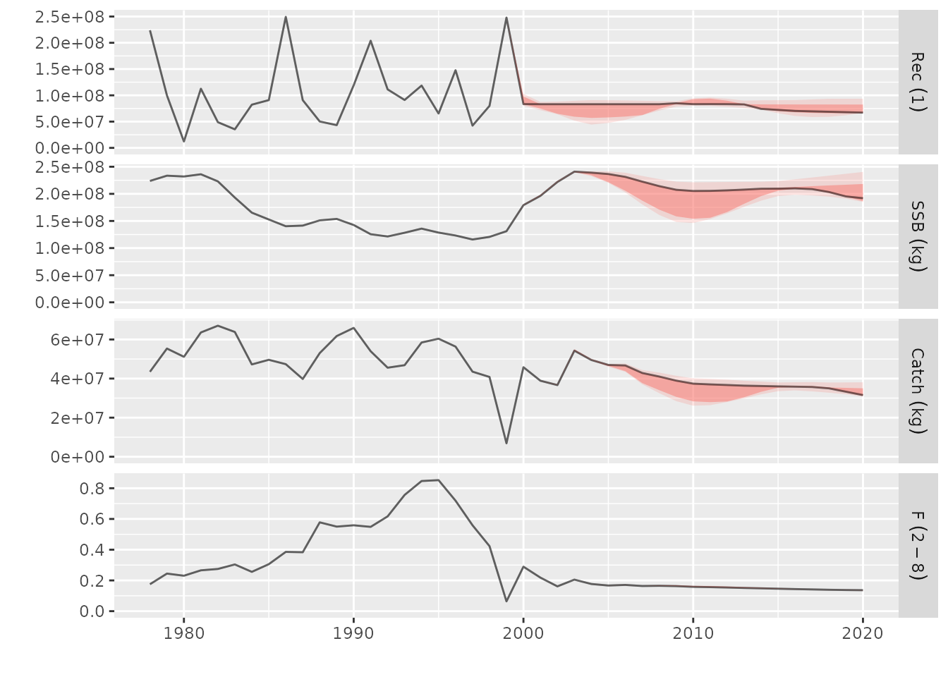
Haddock model prediction using several different stock recruitment models