Run MFDP with a Single Input File

In addition to the classic Lowestoft’s MFDP input data, R MFDP also supports running forecast using a single file for its input data. This new method simplify the run for the users as they can have a quick overview of the data quickly.

Please note you will need to provide a control file if you want to use a single input data file.

The mfdp package provides two samples of the single input files: here. In the same directory you can also find a sample of the control file.

TLDR

For the impatient, here is how to quickly run a forecast using the provided sample files:

# Load library
library(mfdp)

# Get input data path
input_file <- system.file("sample", "nea-had-2020.input.csv", package = "mfdp")
# Get param data path
config_file <- system.file("sample", "nea-had-2020.params.txt", package = "mfdp")

# Reading a single file input must be done in two steps
## Parse the input as FLStock object
input <- read_mfdp_input_table(input_file)
## Run the forecast
output <- mfdp(input, configs = config_file, run_name = "test", out_dir = "out")

For the more detailed descriptions, please continue below.

Input data file structure

The structure of the input data file is identical to the Lowestoft’s MFDP .prd file output. Here is an example of the data:

nea-had-2020.input.csv

"MFDP version 1a"
"Run: Manage2020"
"Time and date: 15:02 27.04.2020"
"Fbar age range: 4-7"
""
""
2020
"Age","N","M","Mat","PF","PM","SWt","Sel","CWt"
3,497416,.402,.027839644,0,0,.276890309,.037,.716
4,531880,.269,.084263959,0,0,.518907563,.154,.95
5,171000,.238,.230460922,0,0,.859979101,.324,1.224
6,60331,.273,.526207605,0,0,1.35966736,.504,1.604
7,29429,.2,.779874214,0,0,1.854188211,.524,1.895
8,10839,.2,.884133612,0,0,2.16838843,.584,2.077
9,9746,.2,.963917526,0,0,2.784901758,.584,2.38
10,3557,.2,.976530612,0,0,3.015625,.584,2.626
11,4436,.2,1,0,0,3.542497377,.584,2.79
12,1896,.2,1,0,0,3.361,.584,3.045
13,4665,.2,1,0,0,3.628,.584,3.329
""
2021
"Age","N","M","Mat","PF","PM","SWt","Sel","CWt"
3,293623,.402,.029,0,0,.269,.037,.708
4,".",.269,.083,0,0,.515,.154,.946
5,".",.238,.215,0,0,.823,.324,1.192
6,".",.273,.457,0,0,1.214,.504,1.471
7,".",.2,.756,0,0,1.774,.524,1.846
8,".",.2,.904,0,0,2.285,.584,2.128
9,".",.2,.948,0,0,2.585,.584,2.311
10,".",.2,.985,0,0,3.222,.584,2.627
11,".",.2,1,0,0,3.416,.584,2.806
12,".",.2,1,0,0,3.726,.584,2.993
13,".",.2,1,0,0,3.677,.584,3.417
""
2022
"Age","N","M","Mat","PF","PM","SWt","Sel","CWt"
3,38636,.402,.029,0,0,.303,.037,.744
4,".",.269,.086,0,0,.526,.154,.957
5,".",.238,.21,0,0,.812,.324,1.182
6,".",.273,.436,0,0,1.168,.504,1.43
7,".",.2,.693,0,0,1.589,.524,1.736
8,".",.2,.888,0,0,2.191,.584,2.087
9,".",.2,.959,0,0,2.718,.584,2.358
10,".",.2,.976,0,0,3.001,.584,2.573
11,".",.2,1,0,0,3.624,.584,2.807
12,".",.2,1,0,0,3.596,.584,3.004
13,".",.2,1,0,0,4.029,.584,3.376
""

"Input units are thousands and kg - output in tonnes"

Control file structure

The control file must be a text file. Here is a sample of the configuration file:

nea-had-2020.params.txt

* example param file for NEA Haddock 2020
Ftarget 0.35 * target F in HCR
Fpa 0.47 * Fpa
Flim 0.77 * Flim
Fagerange 4 7 * age range for reference F (if not given anywhere else)
Bpa 80000 * trigger point in HCR
3yearrule no * use 3-rule in calculating TAC, yes/no
TACpreviousyear 215000 * TAC in intermediate year, used in connection with calculating TAC in first year
maxchangeup 25 * max annual increase in TAC (%)
maxchangedown 25 * max annual decrease of TAC (%)

NOTE: The keywords are case sensitive and all the values are mandatory.

Running the forecast

Running the forecast using the single input is a two-steps procedure:

Loading the data

The first step is we load the data into an FLStock class object:

# Load the mfdp library
library(mfdp)

# Load the input data
input_file <- system.file("sample", "nea-had-2020.input.csv", package = "mfdp")
input <- read_mfdp_input_table(input_file)

print(input)
#> An object of class "FLStock"
#> 
#> Name:  
#> Description:  
#> Quant: age 
#> Dims:  age   year    unit    season  area    iter
#>  11  3   1   1   1   1   
#> 
#> Range:  min  max pgroup  minyear maxyear minfbar maxfbar 
#>  3   13  13  2020    2022    4   7   
#> 
#> catch         : [ 1 3 1 1 1 1 ], units =  NA 
#> catch.n       : [ 11 3 1 1 1 1 ], units =  NA 
#> catch.wt      : [ 11 3 1 1 1 1 ], units =  NA 
#> discards      : [ 1 3 1 1 1 1 ], units =  NA 
#> discards.n    : [ 11 3 1 1 1 1 ], units =  NA 
#> discards.wt   : [ 11 3 1 1 1 1 ], units =  NA 
#> landings      : [ 1 3 1 1 1 1 ], units =  NA 
#> landings.n    : [ 11 3 1 1 1 1 ], units =  NA 
#> landings.wt   : [ 11 3 1 1 1 1 ], units =  NA 
#> stock         : [ 1 3 1 1 1 1 ], units =  NA 
#> stock.n       : [ 11 3 1 1 1 1 ], units =  NA 
#> stock.wt      : [ 11 3 1 1 1 1 ], units =  NA 
#> m             : [ 11 3 1 1 1 1 ], units =  NA 
#> mat           : [ 11 3 1 1 1 1 ], units =  NA 
#> harvest       : [ 11 3 1 1 1 1 ], units =  f 
#> harvest.spwn  : [ 11 3 1 1 1 1 ], units =  NA 
#> m.spwn        : [ 11 3 1 1 1 1 ], units =  NA

You might want to examine the input data to make sure everyting are properly loaded:

# Load the FLCore library
library(FLCore)
#> Loading required package: lattice
#> Loading required package: iterators
#> FLCore (Version 2.6.16.9004, packaged: 2021-09-29 09:21:02 UTC)

# Do checks
print(catch.n(input))
#> An object of class "FLQuant"
#> , , unit = unique, season = all, area = unique
#> 
#>     year
#> age  2020 2021 2022
#>   3  NA   NA   NA  
#>   4  NA   NA   NA  
#>   5  NA   NA   NA  
#>   6  NA   NA   NA  
#>   7  NA   NA   NA  
#>   8  NA   NA   NA  
#>   9  NA   NA   NA  
#>   10 NA   NA   NA  
#>   11 NA   NA   NA  
#>   12 NA   NA   NA  
#>   13 NA   NA   NA  
#> 
#> units:  NA

print(catch.wt(input))
#> An object of class "FLQuant"
#> , , unit = unique, season = all, area = unique
#> 
#>     year
#> age  2020  2021  2022 
#>   3  0.716 0.708 0.744
#>   4  0.950 0.946 0.957
#>   5  1.224 1.192 1.182
#>   6  1.604 1.471 1.430
#>   7  1.895 1.846 1.736
#>   8  2.077 2.128 2.087
#>   9  2.380 2.311 2.358
#>   10 2.626 2.627 2.573
#>   11 2.790 2.806 2.807
#>   12 3.045 2.993 3.004
#>   13 3.329 3.417 3.376
#> 
#> units:  NA

print(stock.n(input))
#> An object of class "FLQuant"
#> , , unit = unique, season = all, area = unique
#> 
#>     year
#> age  2020   2021   2022  
#>   3  497416 293623  38636
#>   4  531880     NA     NA
#>   5  171000     NA     NA
#>   6   60331     NA     NA
#>   7   29429     NA     NA
#>   8   10839     NA     NA
#>   9    9746     NA     NA
#>   10   3557     NA     NA
#>   11   4436     NA     NA
#>   12   1896     NA     NA
#>   13   4665     NA     NA
#> 
#> units:  NA

print(stock.wt(input))
#> An object of class "FLQuant"
#> , , unit = unique, season = all, area = unique
#> 
#>     year
#> age  2020    2021    2022   
#>   3  0.27689 0.26900 0.30300
#>   4  0.51891 0.51500 0.52600
#>   5  0.85998 0.82300 0.81200
#>   6  1.35967 1.21400 1.16800
#>   7  1.85419 1.77400 1.58900
#>   8  2.16839 2.28500 2.19100
#>   9  2.78490 2.58500 2.71800
#>   10 3.01562 3.22200 3.00100
#>   11 3.54250 3.41600 3.62400
#>   12 3.36100 3.72600 3.59600
#>   13 3.62800 3.67700 4.02900
#> 
#> units:  NA

print(ssb(input))
#> An object of class "FLQuant"
#> , , unit = unique, season = all, area = unique
#> 
#>      year
#> age   2020      2021      2022     
#>   all 243130.52   2290.55    339.49
#> 
#> units:  NA

print(fbar(input))
#> An object of class "FLQuant"
#> , , unit = unique, season = all, area = unique
#> 
#>      year
#> age   2020   2021   2022  
#>   all 0.3765 0.3765 0.3765
#> 
#> units:  f

# and so on...

Run forecast using the control file

Now that you are confident that the data is properly loaded, we can continue to run the forecast:

# Get the config file path
config_file <- system.file("sample", "nea-had-2020.params.txt",
                  package = "mfdp")

# Do forecast
output <- mfdp(input, configs = config_file, run_name = "test", out_dir = "out-single")
#> Warning in is.na(raw$stk): is.na() applied to non-(list or vector) of type 'S4'
#> Saving 7.29 x 4.51 in image
#> Saving 7.29 x 4.51 in image
#> Saving 7.29 x 4.51 in image
#> Saving 7.29 x 4.51 in image
#> Saving 7.29 x 4.51 in image
#> Saving 7.29 x 4.51 in image
#> Saving 7.29 x 4.51 in image
#> Saving 7.29 x 4.51 in image
#> Saving 7.29 x 4.51 in image
#> Saving 7.29 x 4.51 in image

Output Files

Running the mfdp function above will instruct MFDP to run the forecast and write output files into ./out directory. We can check the output files:

list.files("out-classic")
#> [1] "test_prm_plot.pdf" "test_prs_plot.pdf" "test-prm.pdf"     
#> [4] "test-prs.pdf"      "test.xlsx"

NOTE: Since we use a control file that contains Fpa, Flim, etc. we are presented with several output files from different F used in the forecast. Note also the summary file that collated the results summary from the runs.

Results

After successfully running a forecast, MFDP returns several output objects in a single list.

The first level will have the sub-list of prm for the Management Options Table and prs for the Single Option Prediction results and
a summary table.

print(names(output))
#> [1] "prm"     "prs"     "summary"

Let’s see the summary from the different F basis:

kableExtra::kable_styling(knitr::kable(output$summary),
            bootstrap_options = "striped", latex_options = "striped")

Basis	Total catch (2021)	F ages 4-7 (2021)	SSB (2022)	% SSB change	% TAC change	% Advice change
fmgmt	232542.8	0.3499983	272206.9	9.070391	8.159432	8.159432
f0	0.0	0.0000000	394626.3	58.122544	-100.000000	-100.000000
fsq	245405.4	0.3731790	265781.1	6.495637	14.142057	14.142057
fpa	296276.8	0.4700000	240776.3	-3.523517	37.803148	37.803148
flim	428699.2	0.7700000	179098.2	-28.237287	99.394955	99.394955

Each prm and prs sub-lists contains the different basis of F used in the forecast.

# Use the F management
print(names(output[["prm"]]))
#> [1] "fmgmt" "f0"    "fsq"   "fpa"   "flim"

# Let's see the Management Options Table for Fmgmt
print(output[["prm"]][["fmgmt"]])
#> $stk
#> An object of class "FLStock"
#> 
#> Name:  
#> Description:  
#> Quant: age 
#> Dims:  age   year    unit    season  area    iter
#>  11  3   1   1   1   21  
#> 
#> Range:  min  max pgroup  minyear maxyear minfbar maxfbar 
#>  3   13  13  2020    2022    4   7   
#> 
#> catch         : [ 1 3 1 1 1 21 ], units =  NA 
#> catch.n       : [ 11 3 1 1 1 21 ], units =  NA 
#> catch.wt      : [ 11 3 1 1 1 21 ], units =  NA 
#> discards      : [ 1 3 1 1 1 21 ], units =  NA 
#> discards.n    : [ 11 3 1 1 1 21 ], units =  NA 
#> discards.wt   : [ 11 3 1 1 1 21 ], units =  NA 
#> landings      : [ 1 3 1 1 1 21 ], units =  NA 
#> landings.n    : [ 11 3 1 1 1 21 ], units =  NA 
#> landings.wt   : [ 11 3 1 1 1 21 ], units =  NA 
#> stock         : [ 1 3 1 1 1 21 ], units =  NA 
#> stock.n       : [ 11 3 1 1 1 21 ], units =  NA 
#> stock.wt      : [ 11 3 1 1 1 21 ], units =  NA 
#> m             : [ 11 3 1 1 1 21 ], units =  NA 
#> mat           : [ 11 3 1 1 1 21 ], units =  NA 
#> harvest       : [ 11 3 1 1 1 21 ], units =  f 
#> harvest.spwn  : [ 11 3 1 1 1 21 ], units =  NA 
#> m.spwn        : [ 11 3 1 1 1 21 ], units =  NA 
#> 
#> $fmult
#> An object of class "FLQuant"
#> iters:  21 
#> 
#> , , unit = unique, season = all, area = unique
#> 
#>      year
#> age   2020           2021           2022          
#>   all 0.99118(0.000) 1.00000(0.741) 1.00000(0.741)
#> 
#> units:  NA 
#> 
#> $ftgt
#> An object of class "FLQuant"
#> iters:  21 
#> 
#> , , unit = unique, season = all, area = unique
#> 
#>      year
#> age   2020       2021       2022      
#>   all 0.37318(0) 0.00000(0) 0.00000(0)
#> 
#> units:  NA 
#> 
#> $parameters
#> $parameters$flag
#> [1] 1 1 3
#> 
#> $parameters$target
#> [1] 215000.00 232543.00      0.35
#> 
#> $parameters$hcrObj
#> $parameters$hcrObj$args
#> $parameters$hcrObj$args$tac
#> [1] 215000
#> 
#> $parameters$hcrObj$args$ftgt
#> [1] 0.35
#> 
#> $parameters$hcrObj$args$fpa
#> [1] 0.47
#> 
#> $parameters$hcrObj$args$flim
#> [1] 0.77
#> 
#> $parameters$hcrObj$args$fbar
#> [1] 4 7
#> 
#> $parameters$hcrObj$args$bpa
#> [1] 80000
#> 
#> $parameters$hcrObj$args$threeYrRule
#> [1] FALSE
#> 
#> $parameters$hcrObj$args$maxTACVar
#> [1] 0.25
#> 
#> $parameters$hcrObj$args$minTACVar
#> [1] 0.25
#> 
#> 
#> 
#> $parameters$ssbunder
#> An object of class "FLQuant"
#> iters:  21 
#> 
#> , , unit = unique, season = all, area = unique
#> 
#>      year
#> age   2020 2021 2022
#>   all 0(0) 0(0) 0(0)
#> 
#> units:  NA

The stk object is an FLStock class object https://flr-project.org/FLCore/reference/FLStock.html from the FLR suite https://flr-project.org/. The developers have provide a wealth of tutorial about the format here: https://flr-project.org/#tutorials.

Next we have the fmult object, which holds the F multiplier values over the years in the FLQuant class, the ftgt object which is the F target over the years, and lastly parameters object, which is the control parameters/configuration for the forecast.

Some example of methods supported by FLStock:

library(FLCore)

# Get the SSB
print(ssb(output[["prm"]][["fmgmt"]]$stk))
#> An object of class "FLQuant"
#> iters:  21 
#> 
#> , , unit = unique, season = all, area = unique
#> 
#>      year
#> age   2020          2021          2022         
#>   all 243131(    0) 249570(    0) 264875(80037)
#> 
#> units:  NA

# Get the Catch total
print(catch(output[["prm"]][["fmgmt"]]$stk))
#> An object of class "FLQuant"
#> iters:  21 
#> 
#> , , unit = unique, season = all, area = unique
#> 
#>      year
#> age   2020           2021           2022          
#>   all 215000(     0) 247226(165771) 240332( 79521)
#> 
#> units:  NA

# Get the Catch number
print(catch.n(output[["prm"]][["fmgmt"]]$stk))
#> An object of class "FLQuant"
#> iters:  21 
#> 
#> , , unit = unique, season = all, area = unique
#> 
#>     year
#> age  2020              2021              2022             
#>   3  14767.05(    0.0)  8793.18( 6462.2)  1157.04(  850.3)
#>   4  66243.10(    0.0) 40281.60(28765.0) 23770.33(16633.2)
#>   5  42064.91(    0.0) 86478.01(59145.6) 52084.48(26082.8)
#>   6  20994.82(    0.0) 34256.37(20699.3) 69694.91(17848.1)
#>   7  10898.65(    0.0) 10389.28( 6142.2) 16256.27( 1784.5)
#>   8   4358.64(    0.0)  5802.15( 3272.4)  5214.05(  554.3)
#>   9   3919.12(    0.0)  2013.61( 1135.7)  2459.93(  293.8)
#>   10  1430.36(    0.0)  1810.56( 1021.1)   853.71(  101.9)
#>   11  1783.83(    0.0)   660.80(  372.7)   767.62(   91.7)
#>   12   762.43(    0.0)   824.10(  464.8)   280.16(   33.5)
#>   13  1875.92(    0.0)  1218.87(  687.4)   866.15(  103.4)
#> 
#> units:  NA

# Get the Fbar
print(fbar(output[["prm"]][["fmgmt"]]$stk))
#> An object of class "FLQuant"
#> iters:  21 
#> 
#> , , unit = unique, season = all, area = unique
#> 
#>      year
#> age   2020           2021           2022          
#>   all 0.37318(0.000) 0.37650(0.279) 0.37650(0.279)
#> 
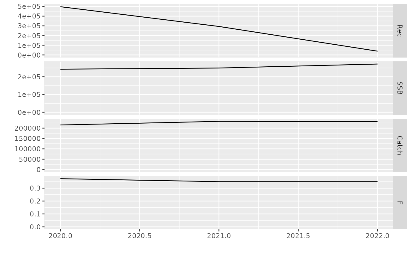
#> units:  f

Let’s plot the forecast results:

# Plot the Management Options Table
plot(output[["prm"]][["fmgmt"]]$stk)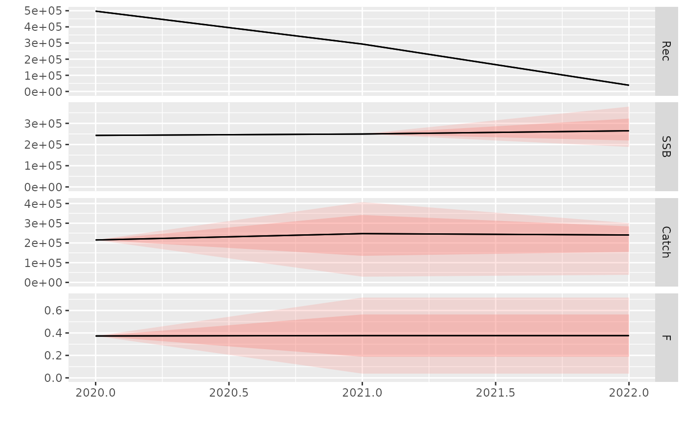

# Single Option Prediction
plot(output[["prs"]][["fmgmt"]]$stk)