Run MFDP with the Classic Input Data

R MFDP supports running forecast using the classic Lowestoft’s MFDP input data. A single input data consists of several files including its index file and a control file. The mfdp package provides samples of these input files here.

Files structure

This set of input files is indexed by an index file. Let’s have a peek at the content in one of the index file (e.g., Fpa2020ind.txt):

Fpa2020ind.txt

Fpa2020MFDP Index file 27.04.2020
 0 
****
Fpa2020CWt.txt
Fpa2020SWt.txt
Fpa2020M.txt
Fpa2020Mat.txt
Fpa2020PF.txt
Fpa2020PM.txt
Fpa2020F.txt
Fpa2020N.txt
Fpa2020Ctrl.txt

The above index file points to several other files. Let’s have a look inside the control file (Fpa2020Ctrl.txt):

Fpa2020Ctrl.txt

HCR2020MFDP Index file 27.04.2020control file27.04.2020
5
4,7
497416,293623,38636,272681,272681,
1
0
0
215000
1.248296
.929582

And one of the data file (Fpa2020CWt.txt)

Fpa2020CWt.txt

Fpa2020CWt
1,3
2020,2024
3,13
1
.716,.95,1.224,1.604,1.895,2.077,2.38,2.626,2.79,3.045,3.329,
.708,.946,1.192,1.471,1.846,2.128,2.311,2.627,2.806,2.993,3.417,
.744,.957,1.182,1.43,1.736,2.087,2.358,2.573,2.807,3.004,3.376,
.744,.957,1.182,1.43,1.736,2.087,2.358,2.573,2.807,3.004,3.376,
.744,.957,1.182,1.43,1.736,2.087,2.358,2.573,2.807,3.004,3.376,

You can find the full description of the files in the official Lowestoft’s MFDP manual document link.

Running the forecast

Running the forecast using the classic input is straightforward:

# Load the mfdp library
library(mfdp)

# Get the index file (note that we need the full path)
input <- system.file("sample/nea-had-2020", "Fpa2020ind.txt", package = "mfdp")
print(input)
#> [1] "/home/runner/work/_temp/Library/mfdp/sample/nea-had-2020/Fpa2020ind.txt"

# Run it
output <- mfdp(input, run_name = "test", out_dir = "out-classic")
#> Warning in readLines(inputfile): incomplete final line found on '/home/runner/
#> work/_temp/Library/mfdp/sample/nea-had-2020/Fpa2020N.txt'
#> Warning in is.na(raw$stk): is.na() applied to non-(list or vector) of type 'S4'
#> Saving 7.29 x 4.51 in image
#> Saving 7.29 x 4.51 in image

Output Files

Running the mfdp function above will instruct MFDP to run the forecast and write output files into ./out directory. We can check the output files:

list.files("out-classic")
#> [1] "test_prm_plot.pdf" "test_prs_plot.pdf" "test-prm.pdf"     
#> [4] "test-prs.pdf"      "test.xlsx"

Results

After successfully running a forecast, MFDP returns several output objects in a single list. Here we use the term prm for the Management Options Table and prs for the Single Option Prediction results.

print(names(output))
#> [1] "prm" "prs"

# Let's see the Management Options Table
print(output[["prm"]])
#> $stk
#> An object of class "FLStock"
#> 
#> Name:  
#> Description:  
#> Quant: age 
#> Dims:  age   year    unit    season  area    iter
#>  11  5   1   1   1   21  
#> 
#> Range:  min  max pgroup  minyear maxyear minfbar maxfbar 
#>  3   13  13  2020    2024    4   7   
#> 
#> catch         : [ 1 5 1 1 1 21 ], units =  NA 
#> catch.n       : [ 11 5 1 1 1 21 ], units =  NA 
#> catch.wt      : [ 11 5 1 1 1 21 ], units =  NA 
#> discards      : [ 1 5 1 1 1 21 ], units =  NA 
#> discards.n    : [ 11 5 1 1 1 21 ], units =  NA 
#> discards.wt   : [ 11 5 1 1 1 21 ], units =  NA 
#> landings      : [ 1 5 1 1 1 21 ], units =  NA 
#> landings.n    : [ 11 5 1 1 1 21 ], units =  NA 
#> landings.wt   : [ 11 5 1 1 1 21 ], units =  NA 
#> stock         : [ 1 5 1 1 1 21 ], units =  NA 
#> stock.n       : [ 11 5 1 1 1 21 ], units =  NA 
#> stock.wt      : [ 11 5 1 1 1 21 ], units =  NA 
#> m             : [ 11 5 1 1 1 21 ], units =  NA 
#> mat           : [ 11 5 1 1 1 21 ], units =  NA 
#> harvest       : [ 11 5 1 1 1 21 ], units =  f 
#> harvest.spwn  : [ 11 5 1 1 1 21 ], units =  NA 
#> m.spwn        : [ 11 5 1 1 1 21 ], units =  NA 
#> 
#> $fmult
#> An object of class "FLQuant"
#> iters:  21 
#> 
#> , , unit = unique, season = all, area = unique
#> 
#>      year
#> age   2020           2021           2022           2023          
#>   all 0.99118(0.000) 1.24830(0.000) 0.92958(0.000) 1.00000(0.741)
#>      year
#> age   2024          
#>   all 1.00000(0.741)
#> 
#> units:  NA 
#> 
#> $ftgt
#> An object of class "FLQuant"
#> iters:  21 
#> 
#> , , unit = unique, season = all, area = unique
#> 
#>      year
#> age   2020       2021       2022       2023       2024      
#>   all 0.37318(0) 0.46998(0) 0.34999(0) 0.00000(0) 0.00000(0)
#> 
#> units:  NA 
#> 
#> $parameters
#> $parameters$flag
#> [1] 1 0 0
#> 
#> $parameters$target
#> [1] 2.150000e+05 1.248296e+00 9.295820e-01
#> 
#> $parameters$ssbunder
#> An object of class "FLQuant"
#> iters:  21 
#> 
#> , , unit = unique, season = all, area = unique
#> 
#>      year
#> age   2020 2021 2022 2023 2024
#>   all 0(0) 0(0) 0(0) 0(0) 0(0)
#> 
#> units:  NA

The stk object is an FLStock class object https://flr-project.org/FLCore/reference/FLStock.html from the FLR suite https://flr-project.org/. The developers have provide a wealth of tutorial about the format here: https://flr-project.org/#tutorials.

Next we have the fmult object, which holds the F multiplier values over the years in the FLQuant class, the ftgt object which is the F target over the years, and lastly parameters object, which is the control parameters/configuration for the forecast.

Some example of methods supported by FLStock:

library(FLCore)
#> Loading required package: lattice
#> Loading required package: iterators
#> FLCore (Version 2.6.16.9004, packaged: 2021-09-29 09:21:02 UTC)

# Get the SSB
print(ssb(output[["prs"]]$stk))
#> An object of class "FLQuant"
#> , , unit = unique, season = all, area = unique
#> 
#>      year
#> age   2020   2021   2022   2023   2024  
#>   all 243131 249570 240780 253928 232520
#> 
#> units:  NA

# Get the Catch total
print(catch(output[["prs"]]$stk))
#> An object of class "FLQuant"
#> , , unit = unique, season = all, area = unique
#> 
#>      year
#> age   2020   2021   2022   2023   2024  
#>   all 215000 296268 210348 190011 152991
#> 
#> units:  NA

# Get the Catch number
print(catch.n(output[["prs"]]$stk))
#> An object of class "FLQuant"
#> , , unit = unique, season = all, area = unique
#> 
#>     year
#> age  2020      2021      2022      2023      2024     
#>   3   14767.05  10929.89   1076.86   8166.03   8166.03
#>   4   66243.10  49400.45  22005.16   3135.95  22074.97
#>   5   42064.91 104111.11  47085.98  30786.24   4054.81
#>   6   20994.82  40517.54  60714.36  41333.86  24811.45
#>   7   10898.65  12255.40  13973.19  32599.65  20222.85
#>   8    4358.64   6805.50   4543.79   8076.07  17157.67
#>   9    3919.12   2361.81   2168.80   2284.02   3687.34
#>   10   1430.36   2123.65    752.67   1090.19   1042.83
#>   11   1783.83    775.07    676.77    378.34    497.75
#>   12    762.43    966.60    247.00    340.19    172.74
#>   13   1875.92   1429.64    763.64    508.02    387.27
#> 
#> units:  NA

# Get the Fbar
print(fbar(output[["prs"]]$stk))
#> An object of class "FLQuant"
#> , , unit = unique, season = all, area = unique
#> 
#>      year
#> age   2020    2021    2022    2023    2024   
#>   all 0.37318 0.46998 0.34999 0.37650 0.37650
#> 
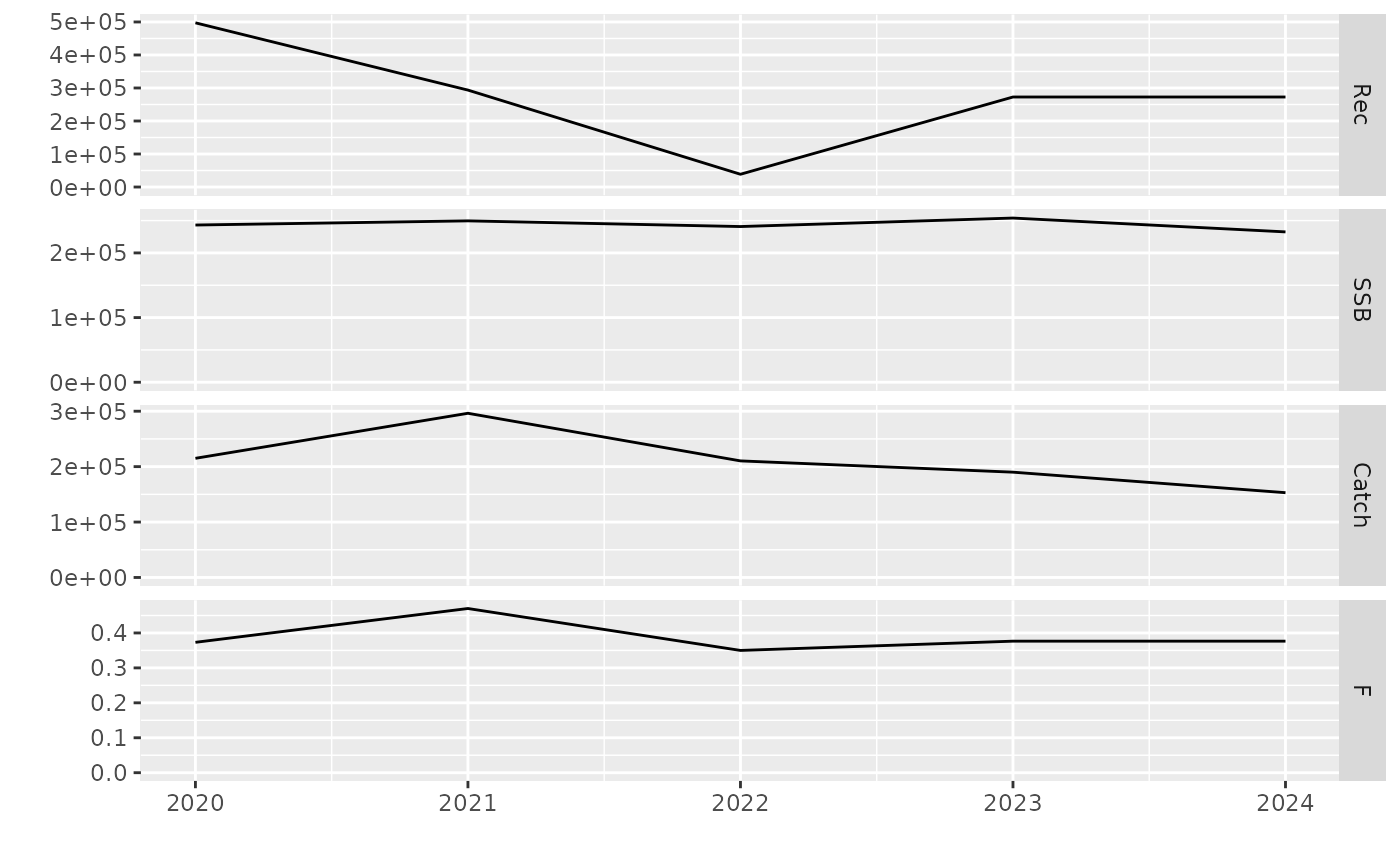
#> units:  f

Let’s plot the forecast results:

# Plot the Management Options Table
plot(output[["prm"]]$stk)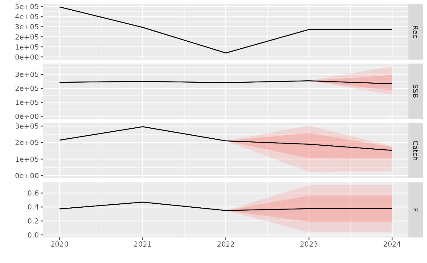

# Single Option Prediction
plot(output[["prs"]]$stk)